How To Make A Cashier Count Chart In Excel : New graphs in Excel 2016 / Introduction to control charts in excel.. When you're ready to create the map chart, select your data by dragging through the cells, open the insert tab, and move to the charts section of the ribbon. A side bar will open in excel for the formatting of the chart. How to make a run chart in excel 1. Whether it is running as expected or there are some issues with it. Now select the pivot table data and create your pie chart as.
You can use the countifs function in excel to count cells in a single range with a single condition as well as in multiple ranges with multiple conditions. Select data and add series 5. If the specific day of the month is inconsequential, such as the billing date for monthly bills. Just select the sales data table, go to insert > chart and hi i have a set of data from pivot table as showin below row labels average of lead time count of title robert. Here we learn how to create a comparison chart in excel and along with examples and a downloadable excel template.
How to create a chart by count of values in Excel? from cdn.extendoffice.com Select chart and click on select data button. Assuming that you want to create a countdown timer until 2020/1/1 in excel, you can do the following steps: Now please follow the steps to finish a control chart. In this tutorial, we learn how to make a histogram chart in excel. Then click on add button and select e3:e6 in series values and keep series name blank. Try to apply the different chart styles, and other options presented in your chart. Select your array of dates (with a header) and create a new pivot chart (insert / pivotchart / ok) then on the field list window, drag and drop the date column in the axis list first and then in the value list first. Next, sort your data in descending order.
You can use the countifs function in excel to count cells in a single range with a single condition as well as in multiple ranges with multiple conditions.
Count formula in excel is used to count the numbers of data in a range of cells, the condition to this formula is that this formula only counts the numbers and no other texts, for example, if we have a formula as =count ( 1, e, 2) then the result displayed is 2 rather than three as the formula only counts the numbers. Speedometer (gauge) chart in excel 2016. Firstly, you need to calculate the mean (average) and standard deviation. Add duration data to the chart. #2 use line charts when you have too many data points to plot and the use of column or bar chart clutters the chart. Control charts are statistical visual measures to monitor how your process is running over a given period of time. Whether it is running as expected or there are some issues with it. Here, reduce the series overlap to 0. Now, let's use excel's replace feature to replace the 0 values in the example. You will also learn how to create the number groups and how to show the % running total in the pivot table. On the insert tab, in the charts group, click the line symbol. I can also use the editing group, on the home tab, to add up, count and find the averages of selections of number data. Perform pareto chart and analysis in excel.
You can use the countifs function in excel to count cells in a single range with a single condition as well as in multiple ranges with multiple conditions. You will also learn how to create the number groups and how to show the % running total in the pivot table. The tiny charts in cell. If i click on cell c22, to make it the active cell, then click on the autosum button in the editing group, the program will enter a formula into the cell. Select the type of chart you want to make choose the chart type that will best display your data.
Download Gantt Chart Excel Wizard | Gantt Chart Excel Template from 1.bp.blogspot.com On the data tab, in the sort & filter group, click za. The tiny charts in cell. Get faster at your task. Click here to download excel file with full interactive chart slider example. Add duration data to the chart. Here, reduce the series overlap to 0. Using a graph is a great way to present your data in an effective, visual way. Get more results from your excel graphs with less effort.
Select chart and click on select data button.
Always have a secondary axis for a combo chart to read better. Here, reduce the series overlap to 0. However, if you can't use excel table for some reason (possibly if you are using excel 2003), there is another (slightly complicated) way to create dynamic chart ranges using excel formulas and named ranges. On the insert tab, in the charts group, click the line symbol. Now, let's use excel's replace feature to replace the 0 values in the example. Next, sort your data in descending order. The map chart in excel works best with large areas like counties, states, regions, countries, and continents. Introduction to control charts in excel. How to make a run chart in excel 1. If the latter, only those cells that meet all of the specified conditions are counted. When you select the chart, the ribbon activates the following tab. This has been a guide to comparison chart in excel. Select chart and click on select data button.
The select data source window will open. You can use the countifs function in excel to count cells in a single range with a single condition as well as in multiple ranges with multiple conditions. First, select a number in column b. In this tutorial, we learn how to make a histogram chart in excel. Create overlay chart in excel 2016.
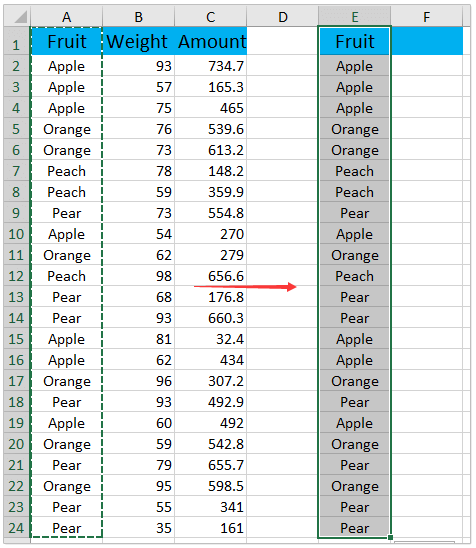
Copying tables and graphs from Excel to Word - YouTube from i.ytimg.com You will also learn how to create the number groups and how to show the % running total in the pivot table. Select the fruit column you will create a chart based on, and press ctrl + c keys to copy. Customize the file or copy the ideas to your work. Click on the series option. On the data tab, in the sort & filter group, click za. Next, sort your data in descending order. If the latter, only those cells that meet all of the specified conditions are counted. Charts are a powerful way of graphically visualizing your data.
This chart is useful to understand that maximum employee
Next, sort your data in descending order. Select data for the chart. Create a control chart in excel. Select your array of dates (with a header) and create a new pivot chart (insert / pivotchart / ok) then on the field list window, drag and drop the date column in the axis list first and then in the value list first. If the latter, only those cells that meet all of the specified conditions are counted. More wacky and fun excel charts Example of control chart in excel; The tiny charts in cell. Perform pareto chart and analysis in excel. Customize the file or copy the ideas to your work. Now, let's use excel's replace feature to replace the 0 values in the example. For example, you have below base data needed to create a control chart in excel. A clustered column chart vs a stacked column chart in excel.

0 Comments:
Posting Komentar